Documentation
I. The Four Axes
There are four indicators that work very nicely together—(a) price-trend, (b) volatility-trend, (c) gamma-ratio, and (d) dark-ratio. Let's describe each as clearly as possible.
P (price-trend)
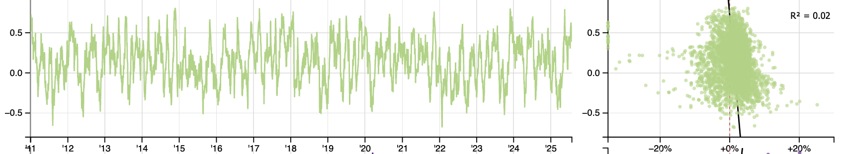 We need a de-trended variable here to show us whether price has been rising or falling recently. Are we trending up or down, and by how much?
Importantly, we want it to be volatility-adjusted, so that a small absolute upside or downside move in conditions of low realized volatility registers the same as a large upside or downside move in high realized volatility. Here's how we do that.

#!/usr/bin/python3

import numpy as np

def period_change(a, n=1):
    chg = ((a - np.roll(a, n)) / np.roll(a, n))
    chg[:n] = np.nan
    return chg

ccr = period_change(closes, 1)		# Day-to-day % changes, 0th = nan
ccv = np.abs(ccr)			# Same-period absolute-ized (volatility)

def moving_average(a, n=21):
    ret = np.cumsum(a, dtype=float)
    ret[n:] = ret[n:] - ret[:-n]
    ret[:n] = np.nan
    return ret / n

ma   = moving_average(ccr, 21)		# 1-month moving average of % changes
mad  = moving_average(ccv, 21)		# 1-month moving average of abs(%)

P = ma / mad				# "price-trend" indicator
The result is an indicator that oscillates primarily between +1 and –1, where +1 suggests that nearly every daily move in the past month was up (–1 indicates down). Since we're normalizing by volatility, this indicator is comparable between time periods as well as between assets.
V (volatility-trend)
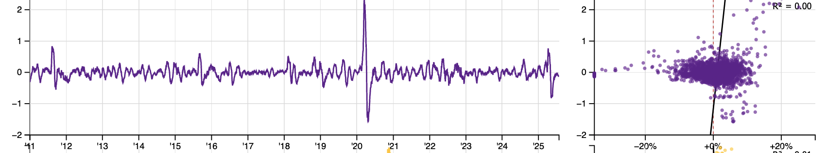 We need another de-trended variable here to show us whether realized volatility has been rising or falling recently. Are we trending up or down, and by how much?

#!/usr/bin/python3

import numpy as np

def period_change(a, n=1):
    chg = ((a - np.roll(a, n)) / np.roll(a, n))
    chg[:n] = np.nan
    return chg

ccr = period_change(closes, 1)		# Day-to-day % changes, 0th = nan
ccv = np.abs(ccr)			# Same-period absolute-ized (volatility)

def moving_average(a, n=21):
    ret = np.cumsum(a, dtype=float)
    ret[n:] = ret[n:] - ret[:-n]
    ret[:n] = np.nan
    return ret / n

ma    = moving_average(ccr, 21)		# 1-month moving average of % changes
mad   = moving_average(ccv, 21)		# 1-month moving average of abs(%)
madMA = moving_average(mad, 21)		# 1-month MA of 1-month MA of abs(%)

V = mad - madMAD			# "volatility-trend" indicator
The result is an indicator that oscillates primarily between +1 and –1, where the units are exactly the same (1-month average daily moves) as with the P indicator.
When V is positive, realized volatility denominated in average daily moves is trending up; and when V is negative, realized volatility denominated in average daily moves is trending down.
G (gamma-ratio)
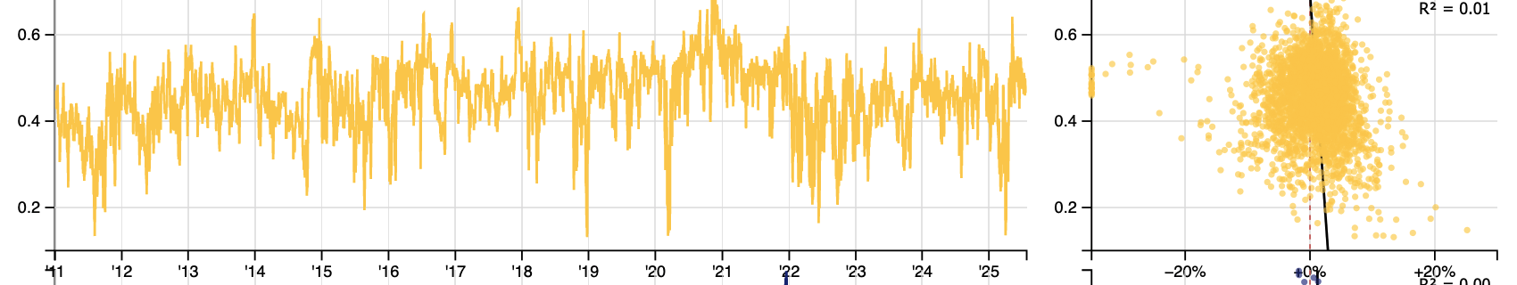 We want to know where there's more call gamma or put gamma, because we want to know whether convexity is leaning toward upside or downside structures. Are we call-driven or put-driven?
Specifically, we want a constant-volatility BSM-delta–derived number, since we want to use a percent gamma (Pgamma), and we don't want to factor in skew or ignore lower-liquidity options.

#!/usr/bin/python3

import numpy as np
from scipy.stats import norm

def delta(cp_flag, S, K, T, r, v):
    d1 = (np.log(S/K)+(r+v*v/2.)*T)/(v*np.sqrt(T))
    if cp_flag == 'c' or cp_flag == 'C':
        return norm.cdf(d1)
    else:
        return -norm.cdf(-d1)

call_gamma = 0
for c in calls:
    delta    = delta('C', c['S'], c['K'], c['T'], 0.00, 0.20)
    up_delta = delta('C', c['S']*1.01, c['K'], c['T'], 0.00, 0.20)
    Pgamma = up_delta - delta
    call_gamma += Pgamma * c['OI']	# multiply by open interest

put_gamma = 0
for p in puts:
    delta    = delta('P', p['S'], p['K'], p['T'], 0.00, 0.20)
    down_delta = delta('P', p['S']*0.99, p['K'], p['T'], 0.00, 0.20)
    Pgamma = down_delta - delta
    put_gamma += abs(Pgamma * p['OI'])	# ensure absolute value of put gamma

total_gamma = call_gamma + put_gamma

G = call_gamma / total_gamma		# "gamma-ratio"
The result is an indicator that moves between 0 and 1, telling us the proportion of call gamma to total gamma. A G of 0.5 means call and put gamma are balanced. A G of 1.0 means it's all calls (0.0 all puts).
D (dark-ratio)
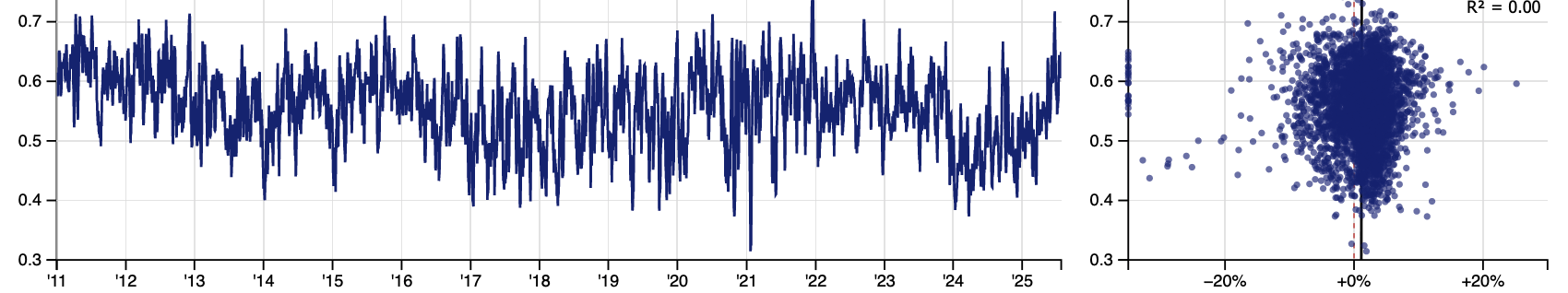 We want to know whether there is more short-selling or long-selling in daily OTC (dark) volume. Generally, short sales are indicative of non-aggressive buying behavior.

#!/usr/bin/python3

import numpy as np

q_short = np.array(load_column("finra_short.csv"))
q_total = np.array(load_column("finra_total.csv"))

dark_ratio = q_short / q_total

def moving_average(a, n=5):
    ret = np.cumsum(a, dtype=float)
    ret[n:] = ret[n:] - ret[:-n]
    ret[:n] = np.nan
    return ret / n

dark_5dma = moving_average(dark_ratio, 5)	# Nice and smooth, but not too smooth
The result is an indicator that moves between 0 and 1, telling us the proportion of short sales in all dark venues over the past week.
II. The Chart
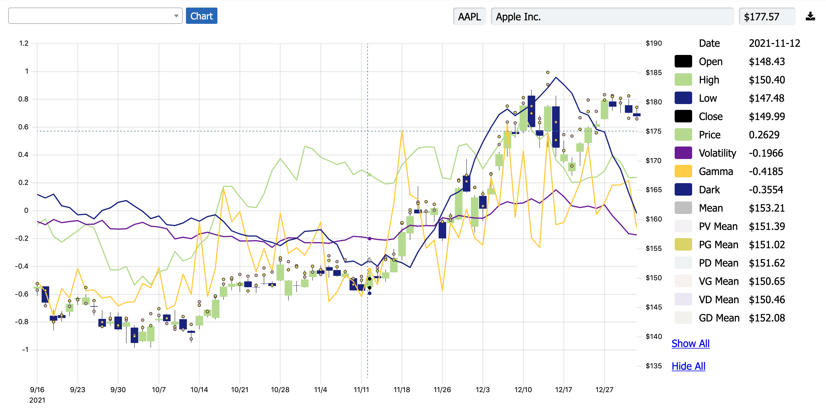
Well, you can just click the "Nearest" button, which runs a k-nearest-neighbor (k-NN) algorithm on each of the four axes to find out which data, historically, is nearest to today's data, and iteratively updates the forecast in the top-right. This is the lazy way.
Or you can take it a step further and try to figure out for yourself what data seems to work and why. To do this, you can click on the "Best" ("Worst") button to see what combination of data has given us the best (worst) performance in the past. Are we currently in a "best" / "worst" scenario? What would it take to get there?
Or you can click-and-drag on the scatterplots yourself, and see how returns change as you home in on a particular combination of data. Add and remove yourself. Take your own slice. What are the characteristics of a given stock? Yes, falling price-trend (P) is bullish for Verizon, but 1-month forward returns double when we combine low P with low G, suggesting that put options play a big role in generating rallies.
Whichever way you want to approach it, there are a few things to keep in mind:
- Use the context plot at the top of the page to test whether patterns have changed over time, and how. You'll notice that higher prices, listed options, and "meme" status can dramatically change the way a stock trades, and which indicators are more predictive. Try looking at discrete timeframes!
- By default, the scatterplots are set to look at 21-day (1-month) returns. You can switch that to 5-day (1-week) by clicking on the 5-day dot in the forecast pane.
- You can change the ticker you're looking at by clicking on the ticker to the left of the stock chart. You can also change the indicators you're looking at by clicking on the letter to the left of the indicator charts—a little drop-down will show up. Right now, we also have IV (1-month ATM straddle) as an option that you can look at.
III. The Sheets (and the API)
Every security in our database can be exported as a spreadsheet document (CSV). Here are the columns in those spreadsheets, and some numerical methods for extending the data:
-
DATE:
YYYY-MM-DD -
P:
The raw 'price-trend' indicator. -
P_NORM:
The normalized 'price-trend' indicator. -
V:
The raw 'volatility-trend' indicator. -
V_NORM:
The normalized 'volatility-trend' indicator. -
G:
The raw 'gamma-ratio' indicator. -
G_NORM:
The normalized 'gamma-ratio' indicator. -
D:
The raw 'dark-ratio' indicator. -
D_NORM:
The normalized 'dark-ratio' indicator. -
IV:
The raw implied volatility, derived from interpolated ATM straddle prices and expressed as an annualized standard deviation (like you're used to). -
IV_NORM:
The normalized implied volatility indicator. -
P_NN:
The historical nearest-neighboring 'price-trend' (P) indicators from the 1/6th (12.5%) of data nearest to today's data (in terms of P, V, G, D, and IV). This is a normalized 1-month price forecast. -
OPEN, HIGH, LOW, CLOSE:
You know how it works. -
VOLUME:
Total (lit and dark tapes) daily volume. -
ADM21:
The 21-day (1-month) average daily move (%). A measure of realized volatility. -
R_21F:
The 21-day (1-month) forward return (%). -
P_21F:
The 21-day (1-month) forward normalized price-trend (P).
All normalization uses a hyperbolic tangent (tanh) function to map a 1-year rolling window of data to the domain [–1, +1].
Learn how to navigate the API here.
IV. The Ideas Page
All securities are presented and automatically sorted by their "P_NN" (the historical price-trends most closely associated with the current data). You're able to change the sorting method, select only bullish (bearish) names, select only rising (falling) names, remove ETFs, or remove short-term-rates-adjacent tickers.
If you have the need to add some complexity to this process, or to apply your own sorting and weighting schemes, there's an API call (/latest) that returns all of the most recent day's data, in JSON or CSV format.